Apply Structural Disorder
Structural disorder in railway tracks can significantly affect the vibration characteristics of the track (see Mantel et al. [2]). This example demonstrates how to set up and run a basic simulation using the Rolland library to calculate the frequency response of different railway tracks with varying structural properties.
Note
This example only determines the track response and the TDR (Track Decay Rate) for a single excitation point! It is recommended to average the results over multiple excitation points to obtain a more accurate representation of the track’s response.
Python Code
1 """
2 Comparative Track Vibration Analysis using Rolland API
3
4 This example demonstrates a comparison of vibration characteristics for:
5 1. Discrete ballasted track (equally spaced mounting positions, equal mounting properties)
6 2. Discrete ballasted track (non-uniform mounting positions, equal mounting properties)
7 3. Discrete ballasted track (non-uniform mounting positions, irregular ballast stiffness)
8 """
9
10 # Import required components from Rolland library
11 from rolland.postprocessing import Response as resp
12 from rolland.postprocessing import TDR
13 from rolland import (
14 ContSlabSingleRailTrack,
15 ContBallastedSingleRailTrack,
16 SimplePeriodicSlabSingleRailTrack,
17 SimplePeriodicBallastedSingleRailTrack, ArrangedBallastedSingleRailTrack, PeriodicArrangement, RandomArrangement
18 )
19 from rolland import DiscrPad, Sleeper, Ballast, ContPad, Slab
20 from rolland import PMLRailDampVertic, DiscretizationEBBVerticConst
21 from rolland import DeflectionEBBVertic, GaussianImpulse
22 from rolland.database.rail.db_rail import UIC60
23
24 # 1. TRACK DEFINITIONS ---------------------------------------------------------
25
26 pad = DiscrPad(sp=[300*10**6, 0], dp=[30000, 0]) # Pad instance
27 sleep = Sleeper(ms=150) # Sleeper instance
28 ball = Ballast(sb=[100*10**6, 0], db=[80000, 0]) # Ballast instance
29 dist1 = 0.6 # 1st sleeper spacing [m]
30 dist2 = 0.7 # 2nd sleeper spacing [m]
31
32 num_mount = 243
33
34 # 1.1 Discrete ballasted track (equally spaced mounting positions, equal mounting properties)
35 track1 = SimplePeriodicBallastedSingleRailTrack(
36 rail=UIC60, # Standard rail profile
37 pad=pad,
38 sleeper=sleep,
39 ballast=ball,
40 num_mount=num_mount, # Number of mounting positions
41 distance=dist1
42 )
43
44 # 1.2 Discrete ballasted track (non-uniform mounting positions, equal mounting properties)
45 track2 = ArrangedBallastedSingleRailTrack(
46 rail=UIC60,
47 pad=PeriodicArrangement(item=[pad]), # No irregularity due to single item
48 sleeper=PeriodicArrangement(item=[sleep]),
49 ballast=PeriodicArrangement(item=[ball]),
50 num_mount=num_mount,
51 distance=PeriodicArrangement(item=[dist1, dist2]) # Periodic alternation of dist1 and dist2
52 )
53
54 # 1.3 Discrete ballasted track (non-uniform mounting positions, irregular ballast stiffness)
55
56 # Generate normal distributed Ballast instances
57 ball_normal = [Ballast(
58 sb=[RandomArrangement.trunc_norm(mean=100, sd=30, minv=70, max_v=130) * 10 ** 6, 0],
59 db=[80000, 0]
60 ) for _ in range(num_mount)]
61
62 track3 = ArrangedBallastedSingleRailTrack(
63 rail=UIC60,
64 pad=RandomArrangement(item=[pad]),
65 sleeper=RandomArrangement(item=[sleep]),
66 ballast=RandomArrangement(item=ball_normal), # Insert list of Ballast instances
67 num_mount=num_mount,
68 distance=PeriodicArrangement(item=[dist1, dist2]),
69 )
70
71 # 2. BOUNDARY CONDITIONS ------------------------------------------------------
72 # Perfectly Matched Layer absorbing boundaries
73 bound = PMLRailDampVertic(l_bound=33.0) # 33.0 m boundary domain
74
75 # 3. EXCITATION SETUP ---------------------------------------------------------
76 # Gaussian impulse at the same position for all tracks
77 x_excit = 71.7 # Excitation position [m]
78 excit = GaussianImpulse(x_excit=x_excit)
79
80 # 4. SIMULATION SETUP & EXECUTION ----------------------------------------------
81 # Discretize and simulate each track type
82 discr1 = DiscretizationEBBVerticConst(track=track1, bound=bound)
83 discr2 = DiscretizationEBBVerticConst(track=track2, bound=bound)
84 discr3 = DiscretizationEBBVerticConst(track=track3, bound=bound)
85
86 defl1 = DeflectionEBBVertic(discr=discr1, excit=excit)
87 defl2 = DeflectionEBBVertic(discr=discr2, excit=excit)
88 defl3 = DeflectionEBBVertic(discr=discr3, excit=excit)
89
90 # 5. POSTPROCESSING & COMPARISON ----------------------------------------------
91 # 5.1 Calculate frequency responses for each track at the excitation point
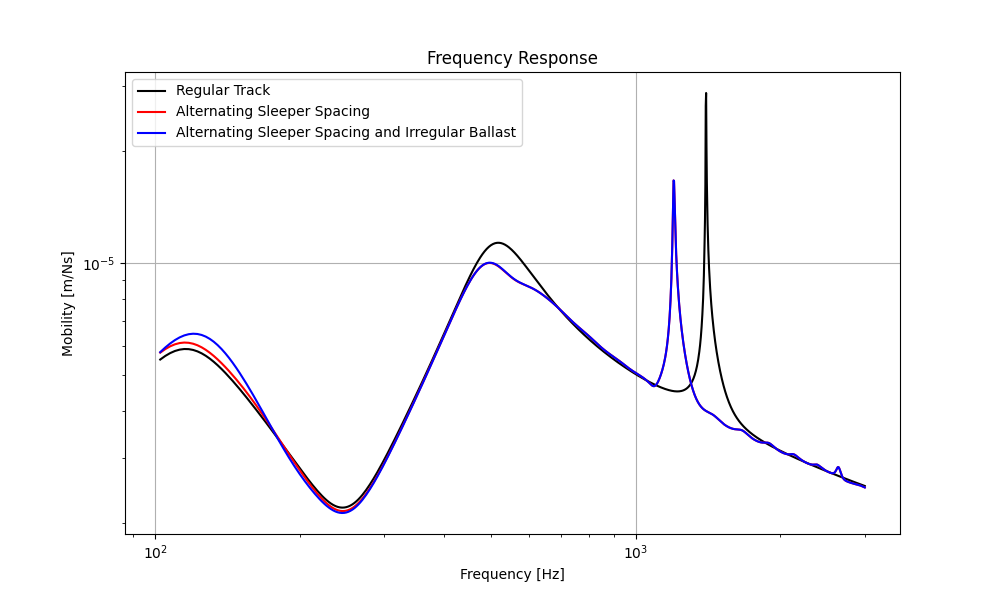
92 pp1 = resp(results=defl1)
93 pp2 = resp(results=defl2)
94 pp3 = resp(results=defl3)
95
96 resp.plot(
97 [(pp1.freq, abs(pp1.mob)),
98 (pp2.freq, abs(pp2.mob)),
99 (pp3.freq, abs(pp3.mob))],
100 ['Regular Track',
101 'Alternating Sleeper Spacing',
102 'Alternating Sleeper Spacing and Irregular Ballast'],
103 title='Frequency Response',
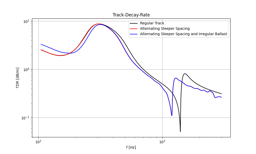
104 x_label='Frequency [Hz]',
105 y_label='Mobility [m/Ns]',
106 )
107
108 # 5.2 Calculate Track Decay Rate (TDR) for each track
109 tdr1 = TDR(results=defl1)
110 tdr2 = TDR(results=defl2)
111 tdr3 = TDR(results=defl3)
112
113 # Plot TDR for each track type
114 TDR.plot([(tdr1.freq, tdr1.tdr), (tdr2.freq, tdr2.tdr), (tdr3.freq, tdr3.tdr)],
115 ['Regular Track',
116 'Alternating Sleeper Spacing',
117 'Alternating Sleeper Spacing and Irregular Ballast'],
118 'Track-Decay-Rate', 'f [Hz]', 'TDR [dB/m]', plot_type='loglog')