First Simulation
This example determines the track response of a double layer track with discrete mounting positions. The track is excited between two sleepers by a Gaussian impulse.
Python Code
1 """
2 Example: Track Vibration Analysis using Rolland API
3
4 This example demonstrates how to:
5 1. Create a railway track model
6 2. Apply excitation and boundary conditions
7 3. Run a vibration simulation
8 4. Analyze and plot the results
9 """
10
11 # Import required components from Rolland library
12 from rolland import DiscrPad, Sleeper, Ballast
13 from rolland.database.rail.db_rail import UIC60 # Standard rail profile
14 from rolland import SimplePeriodicBallastedSingleRailTrack
15 from rolland import (
16 PMLRailDampVertic,
17 GaussianImpulse,
18 DiscretizationEBBVerticConst,
19 DeflectionEBBVertic
20 )
21 from rolland.postprocessing import Response as resp, TDR
22
23 # 1. TRACK DEFINITION ----------------------------------------------------------
24 # Create a ballasted single rail track model with periodic supports
25 track = SimplePeriodicBallastedSingleRailTrack(
26 rail=UIC60, # Standard UIC60 rail profile
27 pad=DiscrPad(
28 sp=[180e6, 0], # Stiffness properties [N/m]
29 dp=[18000, 0] # Damping properties [Ns/m]
30 ),
31 sleeper=Sleeper(ms=150), # Sleeper mass [kg]
32 ballast=Ballast(
33 sb=[105e6, 0], # Ballast stiffness [N/m]
34 db=[48000, 0] # Ballast damping [Ns/m]
35 ),
36 num_mount=243, # Number of discrete mounting positions
37 distance=0.6 # Distance between sleepers [m]
38 )
39
40 # 2. SIMULATION SETUP ---------------------------------------------------------
41 # Define boundary conditions (Perfectly Matched Layer absorbing boundary)
42 boundary = PMLRailDampVertic(l_bound=33.0) # 33.0 m boundary domain
43
44 # Define excitation (Gaussian impulse between sleepers at 71.7m)
45 excitation = GaussianImpulse(x_excit=71.7)
46
47 # 3. DISCRETIZATION & SIMULATION ----------------------------------------------
48 # Set up numerical discretization parameters
49 discretization = DiscretizationEBBVerticConst(
50 track=track,
51 bound=boundary,
52 )
53
54 # Run the simulation and calculate deflection over time
55 deflection_results = DeflectionEBBVertic(
56 discr=discretization,
57 excit=excitation
58 )
59
60 # 4. POSTPROCESSING & VISUALIZATION -------------------------------------------
61 # 4.1 Calculate frequency response at excitation point
62 response = resp(results=deflection_results)
63
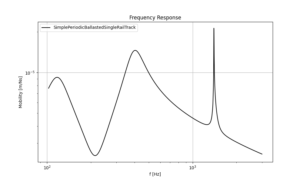
64 # Plot mobility frequency response
65 resp.plot(
66 [(response.freq, abs(response.mob))],
67 ['SimplePeriodicBallastedSingleRailTrack'],
68 title='Frequency Response',
69 x_label='Frequency [Hz]',
70 y_label='Mobility [m/Ns]',
71 )
72
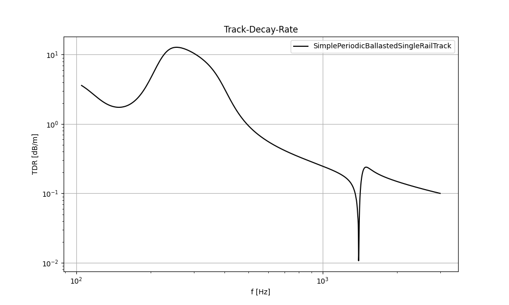
73 #4.2 Calculate Track Decay Rate (TDR)
74 tdr = TDR(results=deflection_results)
75
76 resp.plot([(tdr.freq, tdr.tdr)],
77 ['SimplePeriodicBallastedSingleRailTrack'],
78 title='Track-Decay-Rate',
79 x_label='f [Hz]',
80 y_label='TDR [dB/m]',
81 plot_type='loglog')