Compare Different Tracks
This example demonstrates how to set up and run a basic simulation using the Rolland library to calculate the frequency response of different railway tracks. The example includes continuous and discrete tracks with different with a single or double layer. See [1] for more information.
Python Code
1 """
2 Comparative Track Vibration Analysis using Rolland API
3
4 This example demonstrates a comparison of vibration characteristics for:
5 1. Continuous slab track
6 2. Continuous ballasted track
7 3. Discrete slab track
8 4. Discrete ballasted track
9
10 All tracks are excited with the same Gaussian impulse at 71.7m position.
11 """
12
13 # Import required components from Rolland library
14 from rolland.postprocessing import Response as resp
15 from rolland.postprocessing import TDR
16 from rolland import (
17 ContSlabSingleRailTrack,
18 ContBallastedSingleRailTrack,
19 SimplePeriodicSlabSingleRailTrack,
20 SimplePeriodicBallastedSingleRailTrack
21 )
22 from rolland import DiscrPad, Sleeper, Ballast, ContPad, Slab
23 from rolland import PMLRailDampVertic, DiscretizationEBBVerticConst
24 from rolland import DeflectionEBBVertic, GaussianImpulse
25 from rolland.database.rail.db_rail import UIC60 # Standard rail profile
26
27 # 1. TRACK DEFINITIONS ---------------------------------------------------------
28
29 # 1.1 Continuous slab track
30 cont_slab_track = ContSlabSingleRailTrack(
31 rail=UIC60, # Standard UIC60 rail profile
32 pad=ContPad(sp=[300e6, 0], dp=[30000, 0]), # Stiffness [N/m], damping [Ns/m]
33 l_track=145.2 # Track length [m]
34 )
35
36 # 1.2 Continuous ballasted track
37 cont_ballasted_track = ContBallastedSingleRailTrack(
38 rail=UIC60,
39 pad=ContPad(sp=[300e6, 0], dp=[30000, 0]),
40 slab=Slab(ms=250), # Slab mass [kg]
41 ballast=Ballast(sb=[100e6, 0], db=[80000, 0]), # Ballast properties
42 l_track=145.2
43 )
44
45 # 1.3 Discrete slab track (equally spaced mounting positions)
46 discr_slab_track = SimplePeriodicSlabSingleRailTrack(
47 rail=UIC60,
48 pad=DiscrPad(sp=[180e6, 0], dp=[30000, 0]),
49 num_mount=243, # Number of mounting positions
50 distance=0.6 # sleeper spacing [m]
51 )
52
53 # 1.4 Discrete ballasted track (equally spaced mounting positions)
54 discr_ballasted_track = SimplePeriodicBallastedSingleRailTrack(
55 rail=UIC60,
56 pad=DiscrPad(sp=[180e6, 0], dp=[18000, 0]),
57 sleeper=Sleeper(ms=150), # Sleeper mass [kg]
58 ballast=Ballast(sb=[105e6, 0], db=[48000, 0]),
59 num_mount=243,
60 distance=0.6
61 )
62
63 # 2. BOUNDARY CONDITIONS ------------------------------------------------------
64 # Perfectly Matched Layer absorbing boundaries
65 bound = PMLRailDampVertic(l_bound=33.0) # 33.0 m boundary domain
66
67
68 # 3. EXCITATION SETUP ---------------------------------------------------------
69 # Gaussian impulse at the same position for all tracks
70 x_excit = 71.7 # Excitation position [m]
71 excit = GaussianImpulse(x_excit=x_excit)
72
73 # 4. SIMULATION SETUP & EXECUTION ----------------------------------------------
74 # Discretize and simulate each track type
75 discr1 = DiscretizationEBBVerticConst(track=cont_slab_track, bound=bound)
76 discr2 = DiscretizationEBBVerticConst(track=cont_ballasted_track, bound=bound)
77 discr3 = DiscretizationEBBVerticConst(track=discr_slab_track, bound=bound)
78 discr4 = DiscretizationEBBVerticConst(track=discr_ballasted_track, bound=bound)
79
80 defl1 = DeflectionEBBVertic(discr=discr1, excit=excit)
81 defl2 = DeflectionEBBVertic(discr=discr2, excit=excit)
82 defl3 = DeflectionEBBVertic(discr=discr3, excit=excit)
83 defl4 = DeflectionEBBVertic(discr=discr4, excit=excit)
84
85 # 5. POSTPROCESSING & COMPARISON ----------------------------------------------
86 # 5.1 Calculate frequency responses for each track at the excitation point
87 pp1 = resp(results=defl1) # Continuous slab
88 pp2 = resp(results=defl2) # Continuous ballasted
89 pp3 = resp(results=defl3) # Discrete slab
90 pp4 = resp(results=defl4) # Discrete ballasted
91
92 resp.plot(
93 [(pp1.freq, abs(pp1.mob)),
94 (pp2.freq, abs(pp2.mob)),
95 (pp3.freq, abs(pp3.mob)),
96 (pp4.freq, abs(pp4.mob))],
97
98 ['ContSlabSingleRailTrack',
99 'ContBallastedSingleRailTrack',
100 'SimplePeriodicSlabSingleRailTrack',
101 'SimplePeriodicBallastedSingleRailTrack'],
102
103 title='Frequency Response',
104 x_label='Frequency [Hz]',
105 y_label='Mobility [m/Ns]',
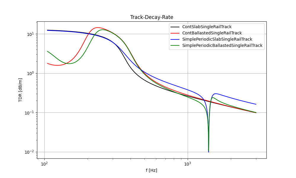
106 )
107
108 # 5.2 Calculate Track Decay Rate (TDR) for each track
109 tdr1 = TDR(results=defl1)
110 tdr2 = TDR(results=defl2)
111 tdr3 = TDR(results=defl3)
112 tdr4 = TDR(results=defl4)
113
114 TDR.plot([(tdr1.freq, tdr1.tdr), (tdr2.freq, tdr2.tdr), (tdr3.freq, tdr3.tdr), (tdr4.freq, tdr4.tdr)],
115 ['ContSlabSingleRailTrack',
116 'ContBallastedSingleRailTrack',
117 'SimplePeriodicSlabSingleRailTrack',
118 'SimplePeriodicBallastedSingleRailTrack'],
119 'Track-Decay-Rate', 'f [Hz]', 'TDR [dB/m]', plot_type='loglog')